Flat, yet deep - How treemaps can be used to visualize complex data
·Before we dive directly into the fun of making treemaps, one word regarding the past, present and future of this blog. The last post I made is around one year ago (so much for the past). Many things have happened in this year, first and foremost that I became father for the second time.
Both family life and my professional life as researcher at Science for Life Lab in Stockholm do in fact leave only limited time for extra activities, like this blog. This is a bit sad for me, but I see it as a temporary issue. I’m still more than dedicated to this blog (present) and will try to post more regularly in the future. Particularly because so many interesting things are happening in the data sciences, and these things have also changed the way I conduct my research and work with data. Just to name of few, I started using github and making my own R packages. I want to write and publish my data analysis pipelines as R markdown notebooks. I want to get more familiar with machine learning, and so on. All of these developments are worth their own posts, but now I start with: treemaps.
What are treemaps? Treemaps are extremely space-efficient yet easy to grasp visualizations for data sets with two important properties: The data can have both numerical and categorial character. The numerical part determines the map in treemap, that means tiles or cells of a 2-dimensional plane are scaled according to the input. Small values become small cells and large values become large cells. The categorial part determines the tree in treemap, that means one big cell can in turn be parent to a set of smaller cells that are nested within it. Well, a picutre is worth a thousand words so let’s look at an example.
Based on existing functions I have compiled an R package for creation of Voronoi and Sunburst treemaps, SysbioTreemaps, available on github and maybe sooner or later on CRAN. Let’s test it.
Installing the package
# install SysbioTreemaps from github
require(devtools)
devtools::install_github("https://github.com/m-jahn/SysbioTreemaps")
# attach packages
library(SysbioTreemaps)
library(tidyverse)
A simple example
We can use the starwars data set from the dplyr package. It’s good
for our purpose because it contains both numeric and categorial data.
The latter are name and home world of the movie characters. The cell
size for each character is encoded by the number of films he or she
showed up in.
df <- dplyr::starwars %>%
  mutate(films = films %>% sapply(length)) %>%
  mutate(name = substr(name, 1, 20)) %>%
  filter(!is.na(homeworld))


# generate voronoi treemap
tm <- voronoiTreemap(
  data = df,
  levels = c("homeworld", "name"),
  cell_size = "films",
  shape = "rounded_rect",
  positioning = "clustered_by_area"
)
## Level 1 tesselation:  0.19 % mean error,  1.45 % max error,  100 iterations
## Level 2 tesselation:  0.64 % mean error,  0.96 % max error,  48 iterations
## Level 2 tesselation:  0.97 % mean error,  0.97 % max error,  58 iterations
## Level 2 tesselation:  0.66 % mean error,  0.99 % max error,  51 iterations
## Level 2 tesselation:  0.66 % mean error,  0.99 % max error,  44 iterations
## Level 2 tesselation:  0.98 % mean error,  0.98 % max error,  28 iterations
## Level 2 tesselation:  0.97 % mean error,  0.97 % max error,  48 iterations
## Level 2 tesselation:  0.38 % mean error,  0.87 % max error,  47 iterations
## Level 2 tesselation:  0.89 % mean error,  0.89 % max error,  39 iterations
## Level 2 tesselation:  0.44 % mean error,  0.93 % max error,  58 iterations
## Treemap successfully created
# draw the treemap
drawTreemap(tm,
  label_level = 1:2,
  label_color = c(grey(0.95), grey(0.85)),
  label_size = c(2, 2)
)
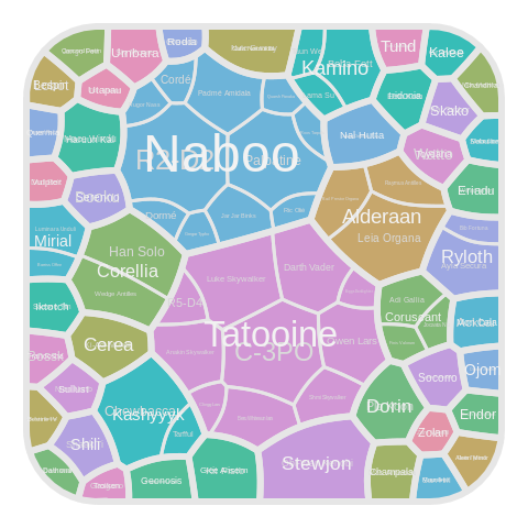
So what happened? In treemap logic, the total area of the plane was subdivided into parental cells and the area of each of these parents corresponds to the sum of the daughter cell’s area. All cells are therefore either directly scaled according to the numerical variable, or aggregated from daughter cells.
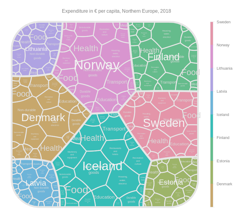
A real world data set
This blog is called Europe by Numbers for a reason. I like to explore data as much as I like to explore European countries. I have often used Eurostat as a source for data regarding European countries, and now there is the fantastic eurostat package for R. We can search for keywords in the description of databases and then download the table of choice. In this example we search expenditures for consumer goods per EU country.
library(eurostat)

# download data from eurostat: we can search for purchasing power parities
search_eurostat("Purchasing power") %>% pull(title) %>% substr(1, 100)
df <- get_eurostat("prc_ppp_ind", type = "label", stringsAsFactors = FALSE)
head(df)
## # A tibble: 6 x 5
##   na_item                ppp_cat               geo             time       values
##   <chr>                  <chr>                 <chr>           <date>      <dbl>
## 1 Nominal expenditure (… Actual individual co… Albania         2018-01-01  10831
## 2 Nominal expenditure (… Actual individual co… Austria         2018-01-01 246801
## 3 Nominal expenditure (… Actual individual co… Bosnia and Her… 2018-01-01  14643
## 4 Nominal expenditure (… Actual individual co… Belgium         2018-01-01 306521
## 5 Nominal expenditure (… Actual individual co… Bulgaria        2018-01-01  38031
## 6 Nominal expenditure (… Actual individual co… Switzerland     2018-01-01 353590
This data set is a time series of consumer goods expenditures from 1995
to 2018, broken down per EU country. We filter the data set for a subset
of interesting variables and countries. Particularly, we filter out
categories (ppp_cat) that seem to be aggregates of sub-categories, for
example ‘Total goods’ et cetera.
# filter for specific year and member country
df_subset <- df %>% filter(
  na_item == "Nominal expenditure per inhabitant (in euro)",
  !grepl("Total|Capital|Gross|[Ff]inal|Actual|Food and|[Cc]ons|serv", ppp_cat),
  time == "2018-01-01"
)

# abbreviate categories
df_subset <- df_subset %>%
  mutate(ppp_cat = substr(ppp_cat, 1, 25) %>% gsub(" ", "\n", .))
Generate treemap and plot it.
# generate voronoi treemap
tm <- voronoiTreemap(
  data = filter(df_subset, geo %in% c("Sweden", "Finland",
    "Denmark", "Iceland", "Estonia", "Lithuania", "Latvia", "Norway")),
  levels = c("geo", "ppp_cat"),
  cell_size = "values",
  shape = "rounded_rect",
  positioning = "clustered_by_area",
  error_tol = 0.001,
  maxIteration = 200
)
## Level 1 tesselation:  0.04 % mean error,  0.1 % max error,  168 iterations
## Level 2 tesselation:  0.05 % mean error,  0.22 % max error,  200 iterations
## Level 2 tesselation:  0.08 % mean error,  0.52 % max error,  200 iterations
## Level 2 tesselation:  0.09 % mean error,  0.46 % max error,  200 iterations
## Level 2 tesselation:  0.1 % mean error,  0.49 % max error,  200 iterations
## Level 2 tesselation:  0.08 % mean error,  0.32 % max error,  200 iterations
## Level 2 tesselation:  0.09 % mean error,  0.59 % max error,  200 iterations
## Level 2 tesselation:  0.13 % mean error,  0.69 % max error,  200 iterations
## Level 2 tesselation:  0.07 % mean error,  0.46 % max error,  200 iterations
## Treemap successfully created
# draw the treemap
drawTreemap(tm,
  label_level = 1:2,
  label_color = c(grey(0.95), grey(0.85)),
  label_size = c(2, 4),
  legend = TRUE,
  title = "Expenditure in € per capita, Northern Europe, 2018"
)
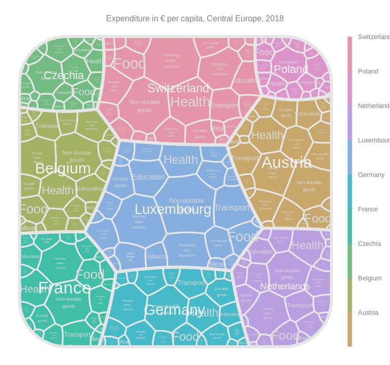
The same thing as it would look for Central Europe…
# trim Germanys name
df_subset <- df_subset %>% mutate(geo = gsub("Germany.*", "Germany", geo))

# generate voronoi treemap
tm <- voronoiTreemap(
  data = filter(df_subset, geo %in% c(
      "Germany", "France", "Poland", "Czechia",
      "Netherlands", "Belgium", "Austria", "Switzerland",
      "Germany (until 1990 former territory of the FRG)",
      "Luxembourg"
    )),
  levels = c("geo", "ppp_cat"),
  cell_size = "values",
  shape = "rounded_rect",
  positioning = "clustered_by_area",
  error_tol = 0.001,
  maxIteration = 200
)
## Level 1 tesselation:  0.04 % mean error,  0.1 % max error,  178 iterations
## Level 2 tesselation:  0.06 % mean error,  0.5 % max error,  200 iterations
## Level 2 tesselation:  0.06 % mean error,  0.46 % max error,  200 iterations
## Level 2 tesselation:  0.09 % mean error,  0.62 % max error,  200 iterations
## Level 2 tesselation:  0.1 % mean error,  0.57 % max error,  200 iterations
## Level 2 tesselation:  0.09 % mean error,  0.51 % max error,  200 iterations
## Level 2 tesselation:  0.15 % mean error,  1 % max error,  200 iterations
## Level 2 tesselation:  0.09 % mean error,  0.39 % max error,  200 iterations
## Level 2 tesselation:  0.1 % mean error,  0.47 % max error,  200 iterations
## Level 2 tesselation:  0.14 % mean error,  0.67 % max error,  200 iterations
## Treemap successfully created
# draw the treemap
drawTreemap(tm,
  label_level = 1:2,
  label_color = c(grey(0.95), grey(0.85)),
  label_size = c(2, 4),
  legend = TRUE,
  title = "Expenditure in € per capita, Central Europe, 2018"
)