Is Sweden smarter than the rest of Europe?

· 08 Apr 2020

The corona virus crisis has overshadowed the life of many EU citizens for quite some time now, and will likely continue to do so for the coming months. The strict social distancing measures taken by many governments leave work places deserted, factories standing still and shops closed. However, one small country on the Northern edge of Europe is going it’s own way to tackle the CoV pandemic and it is highly interesting how this experiment will turn out. None the least as I am part of that experiment.

Note: Original article from 10 April 2020. Figures updated 20 April 2020.

Sweden goes its own way

Many European countries are recently showing signs that the spreading of the virus is slowing down. Countries like Denmark, Germany and Poland went early in lock-down, and started testing more people. Other countries were slower taking social distancing measures ramping up testing. And the UK even made a complete U-turn regarding their strategy, finally introducing stricter social distancing.

Sweden however, where I work and live with my family, decided to implement only mild measures so far, still allowing up to 50 people to gather and not closing any shops. The reasoning here is that people are asked to maintain social distance without enforcing it through authorities. Personal responsibility instead of law and order. Now the big question for everybody living here, but particularly for expats that may have a different view on Swedish society, is if this strategy will work out in the end. This is a highly complex question, because the success of a strategy is not only measured in reduction of virus spread, but also how much burden is put on society and economy. Closed shops and ruined businesses also affect public health, but more indirectly and longer term.

All these questions are hard to answer and will be studied in detail by authorities once the Coronovirus crisis is over. What I want to do here is simply compare how the Swedish strategy of voluntary distancing compares to some of its direct neighbors. For this comparison I’m using data on COVID-19 that the Johns Hopkins University is collecting and sharing on github for public scrutiny and free use. I cloned the repository so that I can access the most recent data and update if neccesary (the repo is updated every day 12 AM).

git clone https://github.com/CSSEGISandData/COVID-19.git

Yet another visualization of CoV spread?

Unfortunately yes. There is hardly a phenomen that got more news coverage than COVID-19, so what’s the point of making one more graph? One motivation is simply to see how the Swedish strategy will turn out in the end (or in the middle, where we are right now). In contrast to all the world maps and bubble charts, I will focus purely on Sweden, and some of its neighboring countries in the EU that partly have similar population size, population density, and health care systems.

# We attach some packages for
# processing and plotting the data
library(tidyverse)
library(lattice)
library(latticeExtra)
library(latticetools)

The first step is to read the *.csv tables for confirmed cases and deaths from the Johns Hopkins University’s data repository. It contains global time series of infections in a ‘wide’ format which is not nice to work with. We need to reshape it to a ‘long’ format as it is more typical for data bases. The long format has all observations of one type in a single column, and all descriptive variables (such as country, or date) in others.

df_world_cases <- read_csv("COVID-19/csse_covid_19_data/csse_covid_19_time_series/time_series_covid19_confirmed_global_20200420.csv")
df_world_death <- read_csv("COVID-19/csse_covid_19_data/csse_covid_19_time_series/time_series_covid19_deaths_global_20200420.csv")

# preview a table
head(df_world_cases[2:5])

## # A tibble: 6 x 4
##   `Country/Region`      Lat   Long `1/22/20`
##   <chr>               <dbl>  <dbl>     <dbl>
## 1 Afghanistan          33    65            0
## 2 Albania              41.2  20.2          0
## 3 Algeria              28.0   1.66         0
## 4 Andorra              42.5   1.52         0
## 5 Angola              -11.2  17.9          0
## 6 Antigua and Barbuda  17.1 -61.8          0

# remove slashes from column names
colnames(df_world_cases) <- colnames(df_world_cases) %>% gsub("/", "_", .)
colnames(df_world_death) <- colnames(df_world_death) %>% gsub("/", "_", .)

# remove greenland and faroe islands from data sets
df_world_cases <- df_world_cases %>% filter(!Province_State %in% c("Greenland", "Faroe Islands"))
df_world_death <- df_world_death %>% filter(!Province_State %in% c("Greenland", "Faroe Islands"))

# select only some countries of interest
countries = c("Sweden", "Finland", "Norway", "Denmark", "Germany", "Poland")
df_world_cases <- filter(df_world_cases, Country_Region %in% countries)[-1]
df_world_death <- filter(df_world_death, Country_Region %in% countries)[-1]

# reshape to long format using gather
# we gather only dates in a single new column
last_date = tail(colnames(df_world_cases), 1)
df_world_cases <- gather(df_world_cases, "date", "cases", "1_22_20":last_date)
df_world_death <- gather(df_world_death, "date", "cases", "1_22_20":last_date)

# now that confirmed cases and deaths are all in one column
# we might as well combine the two dfs in one
df_world <- bind_cols(
  df_world_cases, 
  rename(df_world_death["cases"], deaths = cases)
  )

# parse date-time entries
df_world <- mutate(
  df_world, 
  date = as.POSIXct(strptime(date, format="%m_%d_%y"))
  )

Now that the data is in a handy format for multivariate plotting, we can start to compare cases and fatalities for the selected countries. If I would plot e.g. the confirmed cases on the Y axis on a linear scale, it would be hard to make out differences due to the exponential nature of infectious diseases (2 people infecting each 2 more = 4, then 8, 16, 32, 64, and so on). This is why it is better to plot on a logarithmic axis. Here I chose log 10, so that 1 means 10^1 = 10, 2 = 100, 3 = 1000, 4 = 10,000 and so on).

plot_function = function(metric) {

  xyplot(get(metric) ~ date, 
    df_world %>% filter(date > "2020-02-15"), 
    groups = Country_Region, as.table = TRUE,
    par.settings = custom.lattice(),
    xlab = "", ylab = "log10 cases", main = metric,
    type = "l", lwd = 2, 
    scales = list(y = list(log = 10), x = list(rot = 25, cex = 0.7)),
    yscale.components = yscale.components.log10ticks,
    between = list(x = 0.5, y = 0.5),
    panel = function(x, y, ...) {
      panel.grid(h = -1, v = -1, col.line = grey(0.9))
      panel.xyplot(x, y, ...)
      panel.key(..., points = FALSE)
      # draw labels for the last measured time point
      panel.directlabel(
        x = tail(x, 6), 
        y = tail(y, 6), labels = round(10^tail(y, 6)),
        groups = 1:6, subscripts = 1:6, 
        cex = 0.6, draw_box = TRUE)
      
    }
  )
}

print(plot_function("cases"), split = c(1,1,2,1), more = TRUE)
print(plot_function("deaths"), split = c(2,1,2,1))
grid::grid.text(label = date(), x = 0.15, y = 0.04, 
  gp = grid::gpar(col = grey(0.5), cex = 0.7))

No exponential growth anymore

It is quite clear that Germany is dominating my ‘Northern’ European selection of countries in terms of cases and fatalities. The other countries have lower absolute numbers and also a lower slope of the curve, particularly for the cases. The flattening of the line for all countries means that the disease is not spreading exponentially anymore, but that the rate of new infections is slowing down. This is good. However, the main problem with this representation is that countries with a large population (such as Germany) will always appear on top the figure, although they might take efficient measures to combat spreading of COVID-19.

A fairer representation is not only scaling the data logarithmically, but also normalizing number of cases by population size. This can be easily done by dividing cases and deaths by a new variable population_size. I simply added the number of inhabitants per country in millions, obtained from wikipedia.

# add new variable pop size
df_world <- df_world %>% 
  mutate(population_size = recode(Country_Region,
    Denmark = 5.787725,
    Finland = 5.539832,
    Germany = 83.832481,
    Norway = 5.411798,
    Poland = 37.860731,
    Sweden = 10.088474
    )
  )

# normalize cases and deaths per million of inhabitants
df_world <- mutate(df_world,
    cases_per_million = cases/population_size,
    deaths_per_million = deaths/population_size
  )

print(plot_function("cases_per_million"), split = c(1,1,2,1), more = TRUE)
print(plot_function("deaths_per_million"), split = c(2,1,2,1))
grid::grid.text(label = date(), x = 0.15, y = 0.04, 
  gp = grid::gpar(col = grey(0.5), cex = 0.7))

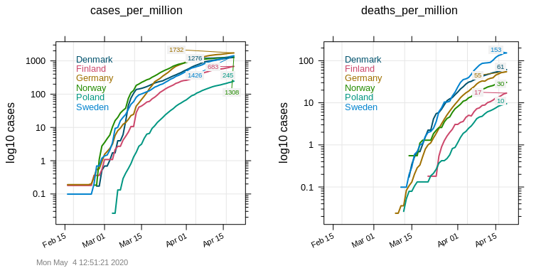
Now the picture looks dfferent. Normalized by population size, the development of new infections over time becomes very similar for all countries except Poland which either managed to control new infections efficiently or is not testing much. For deaths per million inhabitants, Poland has again the lowest number together with Finland. However, here we can suddenly see that Sweden’s fatality numbers are growing more rapidly than the ones of their neighbors, and that by now (last data point: April 9, 2020) Sweden has 10 times more deaths per million inhabitants than Finland.

Too early to draw conclusions

While these numbers somewhat illustrate the different stance Sweden is taking towards COVID-19, it is too early to draw conclusions, or even to request stronger social distancing. It is not clear yet if the higher number of deaths per million inhabitants is purely related to social distancing measures (for sure it is not). It also remains to be seen which long term economic effects the crisis will have on countries with or without lock down. And how that in turn will affect public health, the good that all governments aim to protect now.